Remove The Houston Data Series From The Clustered Bar Chart
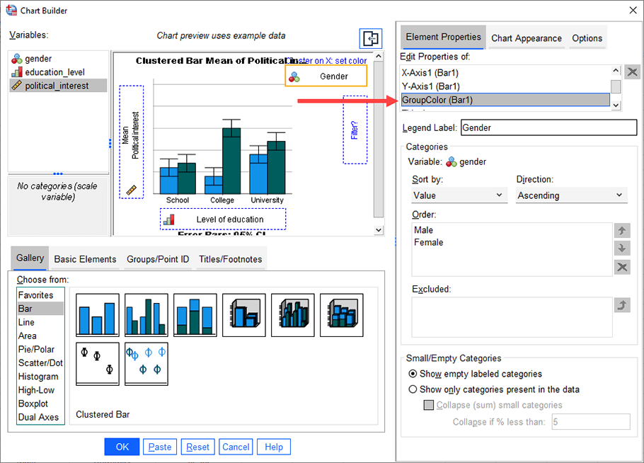
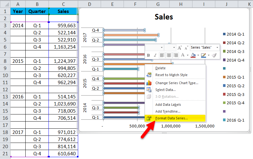
Remove The Houston Data Series From The Clustered Bar Chart - Each different color (each block) has its values in a different column. Filter data in your chart. Web to remove the 'houston' data series from the clustered bar chart, simply click on the bar chart, then on the 'houston' data series to highlight it, and finally press the 'delete' key. View the full answer step 2. To remove the houston data series (range a8:d8) from the clustered bar chart in excel, you will follow these steps: From there, you can choose a “clustered column” chart. Select the bar chart in which you want to. Once we select a chart type, excel will automatically create the chart and insert it into our worksheet. Web removing a data series deletes it from the chart—you can’t use chart filters to show it again. Task instructions х change the pie chart to a clustered bar chart. Task instructions х change the pie chart to a clustered bar chart. Web a clustered column chart displays more than one data series in clustered vertical columns. Clustered columns allow the direct comparison of multiple series, but they become visually complex quickly. From there, you can choose a “clustered column” chart. Each different color (each block) has its values in. Each different color (each block) has its values in a different column. After inserting the chart, you’ll see a bar for each column of your data. Then, find the “charts” group and click on the “recommended charts” option. View the full answer step 2. You can read more about that property of an axis in the api documentation here: Once we select a chart type, excel will automatically create the chart and insert it into our worksheet. Web remove the houston daya series (range a 8:d 8) from the clustered bar chart here’s the best way to solve it. Web in the format data series panel that appears on the right side of the screen, you can adjust the. Web to try it yourself using an existing visual with a clustered column chart, simply follow these three easy steps: Remove the houston data series ( range a 8 :d 8) from the clustered bar chart. Clustered columns allow the direct comparison of multiple series, but they become visually complex quickly. Once you have a chart, you may want to. Web to remove the houston data series from the clustered bar chart, go to the 'design' tab in the chart tools section, click on 'select data', choose the houston data series, and click on 'remove'. Comparing two or more data series has become easier and perhaps more clear with the. Filter data in your chart. Web select the chart and. With your data selected, locate the “insert” tab on the excel ribbon. Web remove the houston daya series (range a 8:d 8) from the clustered bar chart here’s the best way to solve it. Here’s the best way to solve it. Filter data in your chart. They work best in situations where data points are. Here’s the best way to solve it. Each different color (each block) has its values in a different column. Click the chart filters button next to the chart. Web removing a data series deletes it from the chart—you can’t use chart filters to show it again. Web a clustered column chart displays more than one data series in clustered vertical. We can add or remove series and adjust their colors and labels here. If all data series are in contiguous cells, it's easy to just select the chart, and drag the data range selectors to include or exclude. Web removing a data series deletes it from the chart—you can’t use chart filters to show it again. Click the chart filters. Select one series of columns, press ctrl+1 (numeral one) to open the formatting dialog, and in the first screen you see (“series options”) change. Web in the format data series panel that appears on the right side of the screen, you can adjust the following sliders to adjust the spacing of the bars: Let’s start with chart filters. To remove. Next, click on any of the bars in the graph. Post any question and get expert help. Increasing this value will reduce the space between the bars within clusters. Firstly, click on the clustered bar. Each data series shares the same axis labels, so vertical bars are grouped by category. Web in the format data series panel that appears on the right side of the screen, you can adjust the following sliders to adjust the spacing of the bars: You can read more about that property of an axis in the api documentation here: Web to remove the 'houston' data series from the clustered bar chart, simply click on the bar chart, then on the 'houston' data series to highlight it, and finally press the 'delete' key. Firstly, click on the clustered bar. With a few customizations, our clustered bar chart should accurately display our data in an easily understandable format. Select one series of columns, press ctrl+1 (numeral one) to open the formatting dialog, and in the first screen you see (“series options”) change. Each data series shares the same axis labels, so vertical bars are grouped by category. Web removing a data series deletes it from the chart—you can’t use chart filters to show it again. Increasing this value will reduce the space between the bars within clusters. Click ok to apply the changes. Task instructions х change the pie chart to a clustered bar chart. Once we select a chart type, excel will automatically create the chart and insert it into our worksheet. If you want to rename a data series, see rename a data series. We can add or remove series and adjust their colors and labels here. They work best in situations where data points are. Web to remove the houston data series from the clustered bar chart, go to the 'design' tab in the chart tools section, click on 'select data', choose the houston data series, and click on 'remove'.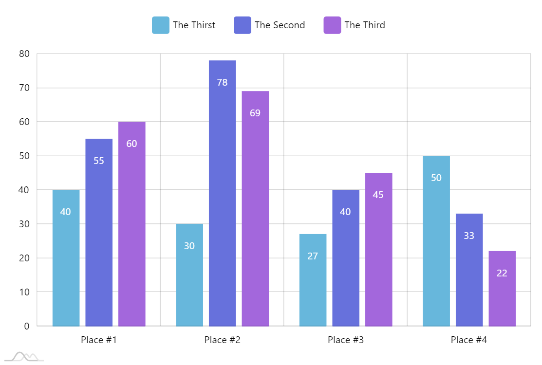
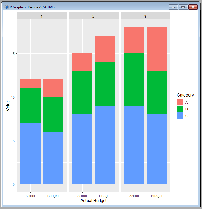
Clustered Bar Chart Amcharts
Clustered Bar Chart
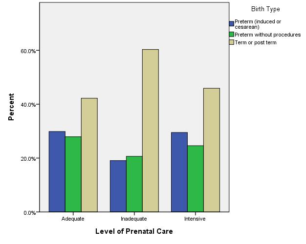
Clustered Bar Chart Spss Chart Examples

Example of clustered bar chart. Download Scientific Diagram
Clustered Bar Chart Spss Chart Examples
Remove The Houston Data Series From The Clustered Bar Chart
Clustered Bar Chart Ggplot Chart Examples
Remove The Houston Data Series From The Clustered Bar Chart
Excel Clustered Bar Chart LaptrinhX

2.1.2.2 Minitab Clustered Bar Chart
View The Full Answer Step 2.
Web To Remove The Houston Data Series From The Gustered Bar Chart, We Need To Select The Houston Data Se.
Clustered Columns Allow The Direct Comparison Of Multiple Series, But They Become Visually Complex Quickly.
Web Reduce The Gap Between Columns/Bars To Give The Chart A Clustered Appearance:
Related Post: